Last year I did some work around EC2 and Tableau Server, and then posted the results of a bunch of tests I carried out to this blog. Since then, I’ve gotten a fair number of questions that essentially ask:
“So, your test results are nice… but what instance type should I run?”
While I’m flattered that people think I’m a “go to” person on the topic, this is a question I really can’t answer – just like I wouldn’t attempt to tell someone who they should or shouldn’t marry or what sort of car to buy. There are way too many variables in play for me to take even a semi-educated stab at these questions.
So if you’ve come here looking for an easy answer, you’ve come to the wrong place. I’m hoping the next couple of posts can give you additional things to think about, however…which will help you make a better informed decision on your own.
The first set of variables to consider encompass you and your workload:
- Number of concurrent users on Tableau Server
- Mix of simple and complex views
- Extract use
The second batch of items reflect the EC hardware resources you have at your disposal to deal with the workload:
- CPU
- Disk
- RAM
AWS neatly packages up RAM and CPU into different instance types for us, so we can simplify a bit:
- CPU & RAM (instance type)
- Disk (storage type)
The tests
In order to have some good data points to discuss, I ran a bunch more tests on various combinations of ec2 instance types and hardware:
EC2 Instance Types:
- c3.xlarge (4 virtual cores, 7.5 GB RAM)
- c3.2xlarge (8 virtual cores, 15 GB RAM)
- c3.4xlarge (16 virtual cores, 30 GB RAM)
- m3.xlarge (4 virtual cores, 15 GB RAM)
- m3.2xlarge (8 virtual cores, 30 GB RAM)
Storage:
- 1 magnetic disk
- 1 general purpose (GP) SSD disk
- 2 GP SSDs striped into a single volume
- 3 GP SSDs striped into a single volume
- 3 EBS SSDs (1500 IOPS each) striped into a single volume
In all cases, I installed the OS to a distinct volume (C: – A single GP SSD). Tableau Server went on D: which represents one of the storage solutions listed above.
I used a low-end skunk works tool to generate the load represented by either two or ten concurrent users on the server (Russell’s definition of “concurrent”: users doing stuff on the server at the same time).
Each of the x users hit the server in parallel, executed 8-9 views over the course of about a minute, and then paused for about 30 seconds before starting all over again. I did this for about 12 minutes for each combination I tested.
Here’s a view of the disk and CPU activity for half of a test– it’s pretty clear when the users are active, and when they’re “resting”.

Between each test I cycled the OS to clear any cached information from RAM. Bouncing the server cleared Tableau’s cache too, needless to say.
Why did I choose 2 and 10 concurrent users? At a ~10% concurrency rate I wanted to try and mimic the type of load a small (< 25 user) and small/medium (< 100 user) server might see. Remember that my workload is different than yours.
[Dear consultant, IT, or technical support person. I’m dropping in this paragraph just for you. When your client tells you that the numbers that they’re seeing don’t match what this blog post promised (even after reading current tongue-in-cheek aside, no less), you are to remind the customer that they are running a different workload than the author. Then, put said client over your knee and spank. Repeat as necessary. Send pictures, too.]
Got that? My workload is different than yours. So your results will be different. The goal of this exercise is to see how the same workload varies in performance across different instance & storage types…not to predict how your workload will behave on these combinations.
My “simple” views consist of a subset of Tableau’s sample reports. Each user also runs a single “complex” dashboard. This dashboard comprises three views which utilize a big-ish 3 GB, 200M row extract. I wanted at least one large extract to drive disk utilization above and beyond the background load one would see from PostgreSQL and loading small extracts from disk for the simple reports.
Now, let’s Talk Storage
Magnetic disks
Don’t use these. Just don’t.
Magnetic disks are cheap because they’re slow. Top line? On average they’re at least 2x slower than 2-striped general purpose SSDs against any complex-ish report.

In the viz above, I’m plotting each report execution as a mark. I’m also attempting to filter out “cached” executions that will artificially drive down average render time by getting rid of any render that took < .4 seconds. Four hundred milliseconds is a somewhat arbitrary guesstimate of how long the fastest “virgin” rendering job might take.
You can see magnetic disks performing (relatively) poorly even with selected reports from the “simple” workload, too:

In all cases above, magnetic = slowest.
Interested in what an unfiltered result looks like (I’ll make all this info available in the next post, BTW)? Here’s the same view with no attempt to remove cached rendering:

Love fio
I used a free disk workbench tool called fio to drive and measure (along with Perfmon) disk performance on the various storage types I tried.
You can download the tool from here: http://git.kernel.dk/?p=fio.git;a=summary
…and the profile I used is here: http://1drv.ms/1zf7Ud3
Make sure that you open up this file and modify the [workload] section to land the disk files the tool creates on the hard disk you wish to test.
FYI, the profile that I’m using executes a mixed 70/30 workload in terms of read/write. Both sequential and random disk access occurs.
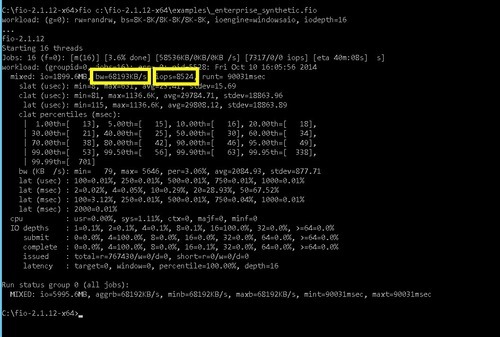
Anyway, here’s what fio tells me about this storage:

We’re getting a lousy 175 IOPS from this disk and 1400 KB/sec disk throughput on the 70/30 read & write workload. That’s 1.4 MB/sec, folks. Would you run ANY application, let alone a Server app on a disk like this? I hope not, because that USB 1.0 thumb drive in the bottom of your junk drawer is about 10x faster by comparison.
Here’s what an execution of a 10 user workload looks like on this disk by way of Perfmon:

We’re using two counters here:
(Blue) Processor – % Processor Time, _Total
(Black) Logical Disk – Average Disk sec / Transfer
Average Disk sec / Transfer is a great disk counter to “cut through the noise” – it measures how long a disk transfer takes. You’ll find a little bit of variation on opinions around what makes for “good” and “bad” value. I think this article represents a pretty happy medium:
http://blogs.msdn.com/b/askjay/archive/2011/07/08/troubleshooting-slow-disk-i-o-in-sql-server.aspx
Counter: Physical Disk / Logical Disk – Avg. Disk sec/Transfer
Definition: Measures average latency for read or write operations
Values: < .005 excellent; .005 – .010 Good; .010 – .015 Fair; > .015 investigate
This disk spends most of it’s life in the “death zone” while vizzes are being rendered. Bad.
General Purpose SSDs
Let’s start off this section with the same workload being executed on the same instance with a single general purpose SSD:

Look at how disk becomes much less of an issue. We get a little bit of “spikeage” when the workload kicks off and that “big” extract gets loaded, but after that, things are pretty clean.

We get 24060 KB/sec throughput (~ 24MB/sec) and 3000 IOPS off this disk….for the moment.
This is important. Read it.
Why in the world did I mention “for the moment”? Well, GP disks are tricky little devils in that they can burst to 3000 IOPS for up to 30 minutes…but then they don’t.
General Purpose SSDs give you a limited “bucket of fast” called “Performance Burst” that you can pull from…and this bucket is replenished over time.
If you don’t “run out of fast”, you’ll be a happy camper. If you do exhaust your fast IO, you revert to the baseline capability of the disk, which is (3 IOPS/sec) * (# GB on the disk). So, a 50 GB General Purpose SSD disk not running in Performance Boost mode is only going to deliver 150 IOPS – not much better than magnetic!
If you want to understand everything about how this works, read the section Under the Hood – Performance Burst Details from the article below:
http://aws.amazon.com/blogs/aws/new-ssd-backed-elastic-block-storage/
This behavior really confused me until I figured out what was going on – while doing my own performance testing, my Tableau Server “suddenly slowed way down for no reason at all” and I couldn’t understand why.
When a customer tells me the same thing I generally think to myself “Yeah, right”. The joke was on me this time.
If your disk usage patterns (low extract usage from what I’ve seen thus far) allow you to leverage the general purpose SSD without “running out of fast” often, it is great, cheap storage. Do make your decision with eyes open, however – you run some risk that your Tableau Server could slow down significantly if your usage patterns change and you exhaust your Performance Boost bucket. If you must have dependable disk performance no matter what, you’ll need EBS volumes with provisioned IOPS.
Striped GP SSDs
Using Windows Disk Management tools, you can stripe multiple ec2 disks of the same size into a single disk on the OS. This is a great way to take multiple smaller GP disks (like a 50 GB SSD) and essentially combine their IOPS under a single drive letter. Striping disks is a standard approach to increasing throughput on PaaS systems.

By striping two disks, I’m doubling my fun in terms of throughput and IOPS. I’m now getting 48,448 KB/sec (~ 48 MB/sec) and 6124 IOPS. This technique is getting me into the neighborhood of the performance of one of the physical SSDs I have running at home might deliver:
What does report execution look like on this 2 striped GP SSDs? Disk is pretty smooth, even when we load the extract:

Lets take a look at our vizzes again. Note how the 2 striped SSDs are far and away the performance leader when it comes to rendering a complex viz. For “simple” workloads, it appears disk is less of an issue.
 If two striped disks is good, three must be even better, right? Yes. We see 70,421 KB/sec (70.4 MB/sec) throughput and 8802 IOPS – all three disks are obviously running in Performance Boost mode right now.

We see no big “spikes” of IO here, either:

This extra disk does improve rendering performance, but only moderately… and for the most expensive (max reference line) vizzes we’re rendering in each category:

Based on my personal workload it looks like we’re approaching the point of diminishing returns in turns of adding extra IO, so I’m going to stop now as I don’t want to spend $$ on disk that doesn’t do anything for me.
Striped EBS Volumes
One can stripe EBS disks, too. EBS disks allow you to reserve “provisioned” IOPS so that you always have the disk that you need. Essentially, this is guaranteed IO, and you’re going to pay for it whether you use it or not.
The advantage of EBS disks with provisioned IOPS is obvious – your IO throughput needs will always be met, every time …assuming you grabbed enough IOPS when you configured the disks.
The disadvantage is that you’re not going to get that neat Performance Burst mode that lets them burst to 3000 IOPS. If you WANT to burst at 3000 IOPS, you have to set the disks to provide that level of service all the time.
In the test below, I created three 50 GB EBS disks, each with 1500 provisioned IOPS. Based on what we’ve seen before, I expect to see about 4500 IOPS from the volume on my OS. EBS delivers:

Note that my 2 striped GP disks offer better performance while they are able to burst…but they won’t always be able to burst, which is the whole point.
Disk latency looks like we’d expect it to since we’re working with less (but more dependable) throughput.

And of course, we would expect a bit of a drop in rendering performance, which we can see here:

Summary
What have we learned?
- Disk matters. Different storage can impact Tableau Server rendering performance on the same ec2 instance type
- Magnetic disk = poor performance.
- Use magnetic storage and you will be miserable
- General Purpose SSDs offer reasonably priced performance and are great while in Performance Boost mode
- If you “run out of fast” and your GP SSD reverts to baseline mode, performance can quite suddenly begin to suffer.
- Striping disks is how to “stack” IOPS to improve throughput
- EBS disks let you dial in the amount of throughput you need – and you pay for that amount all the time.
When it comes time to decide how to configure your storage, I’d suggest you run the two Performance Monitor counters mentioned earlier to get an idea of what your IO workload looks like. You want to try and keep that Average Disk sec / Transfer counter under 10-15 ms.
If your workload is “bursty”, general purpose SSDs could be a great solution. If you need steady IO all the time, think about EBS disks.
Next up – Let’s compare average rendering time based on different combinations of disk & instance type. Woo-hoo!